Calculus I · The Mean Value Theorem

Now tilt it: the Mean Value Theorem

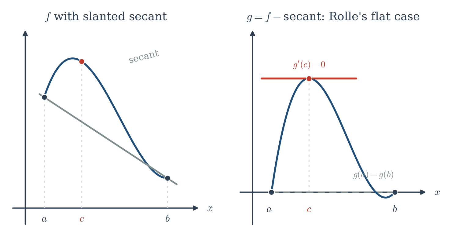
Rolle handled the flat case, where the endpoints are level. The Mean Value Theorem handles every case by a trick so good it’s almost cheating: tilt the whole picture until the endpoints are level, apply Rolle, then tilt back.

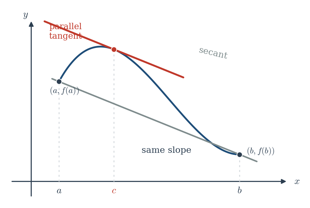
Mean Value Theorem. If $f$ is continuous on $[a,b]$ and differentiable on $(a,b)$, then there is at least one point $c$ in $(a,b)$ where $$f'(c) = \frac{f(b) - f(a)}{b - a}.$$

The right side is the average rate of change over the whole interval — the slope of the straight “secant” line connecting the two endpoints of the graph. The theorem says some interior tangent line is parallel to that secant: at the instant $c$, your instantaneous rate equals your trip average. (Figure 6.2: the secant line through the endpoints, and a parallel tangent line touching the curve at $c$.)

◆ Proof of the MVT

Subtract off the secant line to flatten the endpoints. Define $$g(x) = f(x) - \left[\,f(a) + \frac{f(b)-f(a)}{b-a}\,(x - a)\right].$$ The bracket is exactly the secant line, so $g$ measures how far $f$ sits above or below it. Check the endpoints: $g(a) = f(a) - f(a) = 0$, and $g(b) = f(b) - f(b) = 0$. So $g(a) = g(b)$, and $g$ inherits continuity and differentiability from $f$. Rolle applies to $g$: there’s a $c$ with $g'(c) = 0$. But $$g'(x) = f'(x) - \frac{f(b)-f(a)}{b-a},$$ so $g'(c) = 0$ means precisely $f'(c) = \dfrac{f(b)-f(a)}{b-a}$. $\blacksquare$

Notice what just happened: the general theorem cost us almost nothing once we had the special one, because subtracting a straight line changes slopes by a constant and converts “average slope” into “zero.” That move — straighten the problem, solve the easy version, un-straighten — is one you’ll use for the rest of your mathematical life.

Why this chapter exists: three consequences

The MVT is a tool, and here is what it builds. Each of these is short to prove now and impossible to prove without it.

Consequence 1 — Zero slope means constant (the Chapter 5 debt, repaid)

If $f'(x) = 0$ at every point of an interval, then $f$ is constant on that interval.

Proof. Take any two points $x < y$ in the interval. By the MVT, $f(y) - f(x) = f'(c)\,(y - x)$ for some $c$ between them. But $f'(c) = 0$, so $f(y) - f(x) = 0$, i.e. $f(y) = f(x)$. Every two points have the same value: $f$ is constant. $\blacksquare$

This looks almost too obvious to need proving — of course a function that never changes is constant. But “never has slope” and “never changes value” are genuinely different statements, and the only bridge between them is the MVT. Back in Chapter 5 we wanted to show $Ce^{kx}$ was the solution to $\frac{dN}{dt} = kN$, not merely a solution, and the whole argument hinged on “$g'(x) = 0$ everywhere, therefore $g$ is constant.” We used it on faith. That loan is now paid in full.

A twin fact comes for free and will run all of integration: if $f'(x) = g'(x)$ everywhere, then $f$ and $g$ differ by a constant (apply Consequence 1 to $f - g$). When you reach Chapter 10 and wonder where the “$+C$” in an antiderivative comes from — this is its birth certificate.

Consequence 2 — The sign of the derivative controls rising and falling

If $f'(x) > 0$ on an interval, then $f$ is increasing there. If $f'(x) < 0$, then $f$ is decreasing.

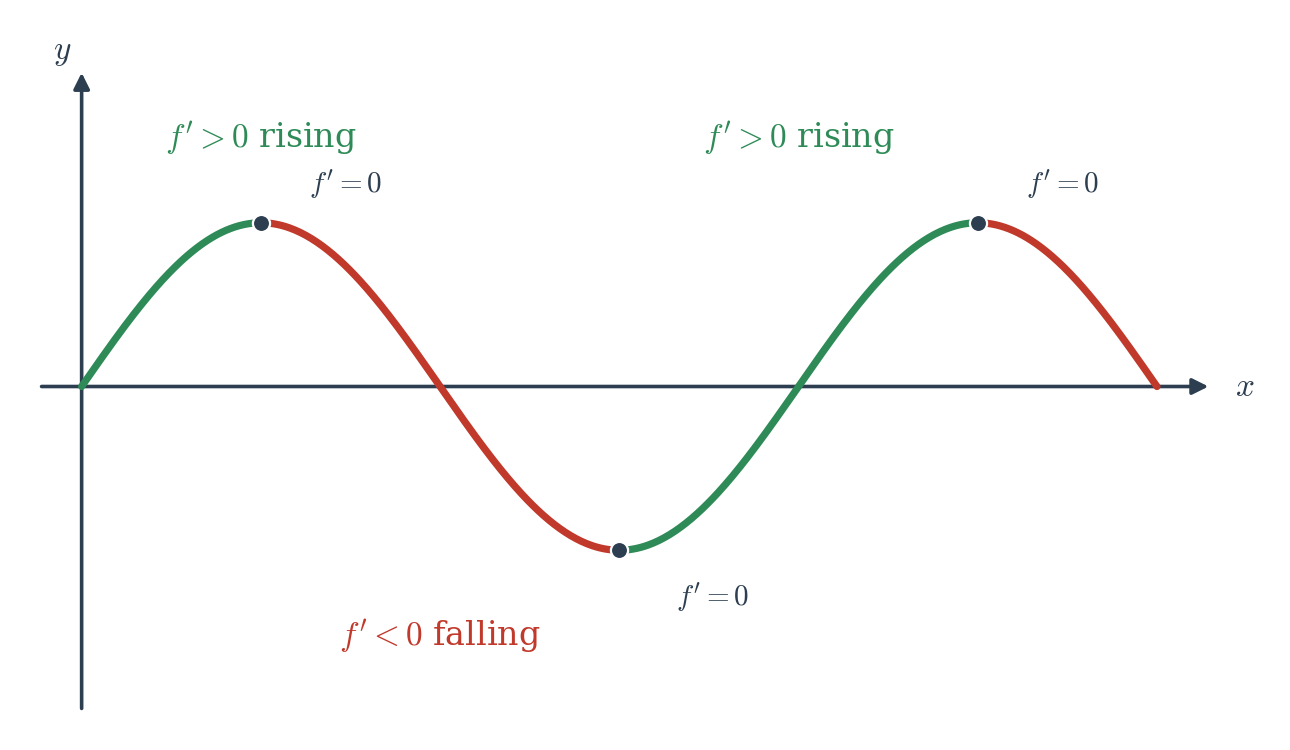
Proof. Take $x < y$. The MVT gives $f(y) - f(x) = f'(c)(y - x)$ with $y - x > 0$. If $f'(c) > 0$ the right side is positive, so $f(y) > f(x)$: increasing. If $f'(c) < 0$, it’s negative, so $f(y) < f(x)$: decreasing. $\blacksquare$

This is the one that earns its keep in Chapter 8. The entire method of finding maxima and minima — locate where $f'$ changes sign, because that’s where $f$ turns around — is just this consequence, read carefully. Without it, “set the derivative to zero” would be a ritual with no justification. With it, it’s a theorem.

Consequence 3 — A function can’t outrun its steepest slope

If $|f'(x)| \le M$ everywhere on $[a,b]$, then $|f(b) - f(a)| \le M\,(b - a)$.

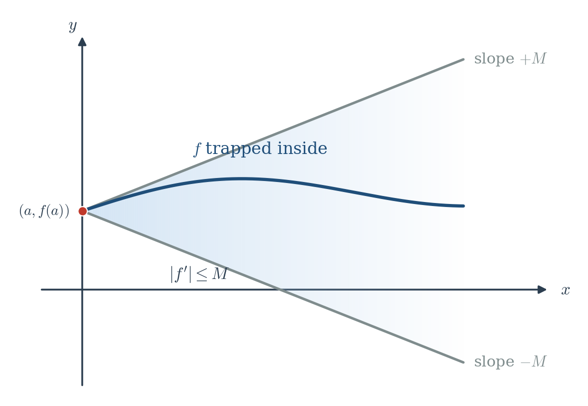
Proof. By the MVT, $f(b) - f(a) = f'(c)(b-a)$, so $|f(b) - f(a)| = |f'(c)|\,(b-a) \le M(b-a)$. $\blacksquare$

This is the rigorous version of the robustness idea from Chapter 2: a function whose slope is capped simply cannot change too much over a short interval. It is the reason numerical methods come with error guarantees — bound the derivative, and you’ve bounded how wrong you can be. Engineers live on inequalities like this one.

◆ Layer 2 — The generalized MVT, and a glimpse of Taylor’s engine

There’s a two-function version of the MVT, due to Cauchy, that looks technical but is the secret machinery behind Chapter 7’s Taylor remainder (and behind L’Hôpital’s rule, if you meet it).

Cauchy’s MVT. If $f$ and $g$ are continuous on $[a,b]$ and differentiable on $(a,b)$, there is a $c$ in $(a,b)$ with $$\big[f(b) - f(a)\big]\,g'(c) = \big[g(b) - g(a)\big]\,f'(c).$$ Proof (same tilt trick, cleverer line). Apply Rolle to $h(x) = \big[f(b)-f(a)\big]g(x) - \big[g(b)-g(a)\big]f(x)$. A quick check gives $h(a) = h(b)$ (the cross terms cancel), so some $c$ has $h'(c) = 0$, which is exactly the claim. $\blacksquare$

Why care now? The ordinary MVT says $f(b) = f(a) + f'(c)(b-a)$ — it pins down $f$ at $b$ using one derivative and an unknown midpoint $c$. Taylor’s theorem will say $f(b) = f(a) + f'(a)(b-a) + \tfrac12 f''(c)(b-a)^2$ — the same shape, one derivative deeper, and Cauchy’s MVT is what proves that error term has exactly that form. The MVT isn’t just a theorem in this book; it’s the first rung of a ladder.

All 12 chapters of Calculus I · Foundations · All courses