A First Taste of Algorithms · Two Questions
Counting the halvings
So binary search costs “however many times you can halve the list before nothing is left.” Give that a name and a table. Start with n items; each comparison cuts the living region at least in half:
| items n | comparisons needed (worst case) |
|---|---|
| 8 | 4 |
| 100 | 7 |
| 1,000 | 10 |
| 1,000,000 | 20 |
| 1,000,000,000,000 | 40 |
Read the table the way you read the race in Lab 1: the left column is multiplying — by 10, by 1000 — and the right column is adding a handful each row. A thousand times more items costs ten more comparisons. You met the function that behaves this way in Book 2: the logarithm, the function that turns multiplication into addition. The number of halvings from n down to 1 is log₂ n, give or take a rounding we’ll pin down in the deep water — and that is why a trillion-item phone book for the whole galaxy would surrender any name in forty questions. Forty. You could do it at a kitchen table before the tea cools.
When the cost of a procedure grows like n, we call it linear; like log n, logarithmic. For now these are just names for shapes you have seen in your own tables — the steady ramp and the nearly-flat curve. We will not dress them in formal notation until Chapter 6, when we’ll have enough tables behind us that the notation arrives as bookkeeping instead of vocabulary.
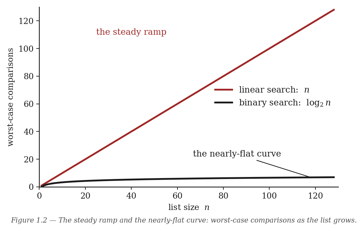
Figure 1.2 — The steady ramp and the nearly-flat curve: worst-case comparisons as the list grows.
One more honest note, because this book does not hide its bills. Binary search demands a sorted list, and lists are not born sorted. Sorting costs something. How much, exactly — and whether anything could ever sort faster — is Chapter 6’s story, and it ends with the most surprising kind of theorem in this book: a proof that something is impossible. Whether the toll is worth paying depends on how many searches you’ll run afterward, which is the kind of answer cost questions usually have: not “yes” or “no” but “it depends, and here is precisely on what.”
Deeper water: the invariant
Here is the correctness argument for binary search, done properly. Through the entire procedure, maintain this sentence:
If the target is in the list at all, it lies between the two fingers.
A sentence kept true through every step of a procedure is called a loop invariant, and proving one is always the same three moves — the same three moves, you’ll notice, as induction in Book 2, because it is induction, marching over steps of a procedure instead of whole numbers:
- It starts true. Before any comparison, the fingers bracket the whole list. If the target is anywhere, it’s in there. ✓
- Each step keeps it true. Suppose it’s true going into a comparison, and the middle item is too small. Sortedness says everything from the middle leftward is also too small, so the target — if present — was already in the right portion. Moving the left finger past the middle discards only dead territory. The sentence survives. (The too-big case is the mirror image.) ✓
- It’s true at the end, and that finishes the job. The procedure stops in one of two ways. If it finds the target — correct, trivially. If the fingers cross, the invariant says: the target, if present, lies in a region that no longer exists. So it isn’t present, and saying so is correct. ✓
Notice what step 3 bought: the proof of absence. The invariant is why binary search’s “not here” is a theorem, not a shrug. Hold the method itself, too — start true, stays true, finishes the job — because every correctness proof in this book is this argument wearing different clothes.
Deeper water: the exact count
“About log₂ n” can be made exact. With k yes/no questions, the answers form a sequence like yes, no, no, yes… — and there are exactly 2ᵏ such sequences. Each possible position of the target must lead to a different answer-sequence (if two positions produced identical answers, the procedure couldn’t tell them apart — it would answer at least one of them wrongly). A list of n items has n + 1 distinguishable situations: “it’s at position 1,” …, “it’s at position n,” and “it’s absent.” So we need 2ᵏ ≥ n + 1, that is,
k ≥ log₂(n + 1), so k = ⌈log₂(n + 1)⌉ questions suffice and are required
(the brackets mean “round up”). Check it against the table: n = 1,000,000 gives log₂(1,000,001) ≈ 19.93, round up to 20. ✓
Read the argument once more, because something remarkable just happened: it doesn’t mention binary search. It says no questioning strategy whatsoever — however clever, however different from halving — can beat ⌈log₂(n+1)⌉ in the worst case. You have just seen your first lower bound: a fence around what is possible, proved by counting answer-sequences rather than by trying strategies. Chapter 6 builds its great impossibility theorem with exactly this kind of fence.
A human moment
Binary search was first published in 1946, in the earliest days of electronic computers. Here is the astonishing part, reported by Jon Bentley and documented by Donald Knuth: the first published version that worked correctly for every list length did not appear until 1962. For sixteen years, the cleverest people alive wrote this twelve-line procedure with small bugs at the edges — fingers crossing wrongly, regions of size one mishandled. And the story isn’t over: in 2006 an engineer at Google discovered that the binary search shipped inside Java, used by millions of programmers for two decades, broke on sufficiently huge lists — the innocent line computing the middle could overflow the machine’s fixed-size numbers. (Python’s numbers grow as needed, so your Lab 1 version is safe; the lesson isn’t.) Hold both facts next to the deep water above. The invariant proof is short, and it is the only reliable defense humanity has found against sixteen years of off-by-one — which is why Break-it 1 in the lab, where you sabotage
+ 1and watch, is not a toy exercise but a reenactment.
All 32 chapters of A First Taste of Algorithms · Foundations · All courses