A First Taste of Algorithms · Building the Learner

Weighted looking-back

One idea separates the toy above from the architecture — the transformer — behind the systems you actually use, and it is simple enough to state plainly and honest enough to deserve stating. The toy looks back at a fixed few characters. The transformer looks back at all of them, but learns how much to weigh each one for the prediction at hand. Guessing the letter after “riema—”, the model has learned to weigh the “r” and the “m” heavily and the earlier letters less; guessing after a different stem, it weighs differently. Each position asks every earlier position “how much do you matter to what comes next?”, and the weights — which sum to one, the softmax of Chapter 8 turning raw scores into proportions — are not hand-set but learned, by the same descent, priced by the same backward sweep.

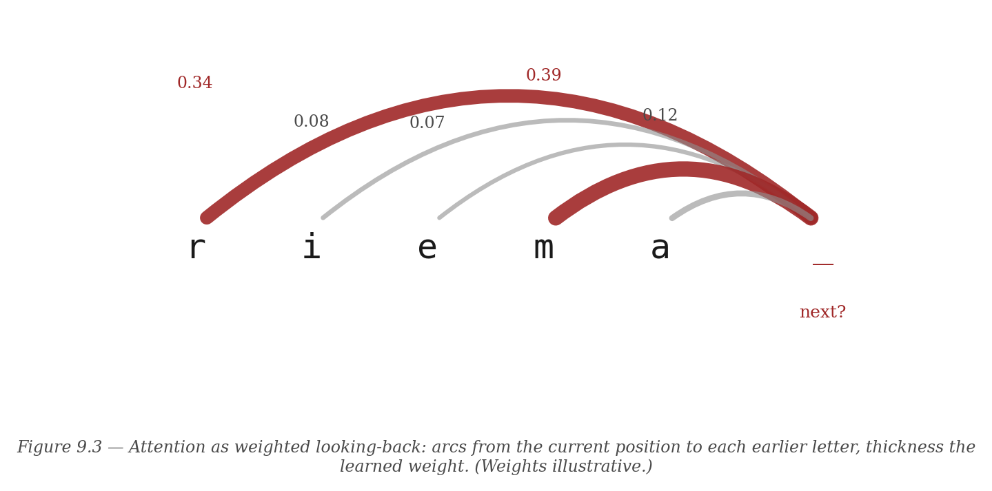
Figure 9.3 — Attention as weighted looking-back: arcs from the current position to each earlier letter, thickness the learned weight — the model’s own opinion about which letters matter for what comes next.

That is attention: weighted looking-back, with the weights learned. Stack a few layers of it, train on enough text instead of just names, and the same machine you built for mathematicians becomes the same species of machine — differing in size and data, not in kind — that completes your sentences and answers your questions. There is no further secret. There is more engineering than any one person holds, and vastly more data and electricity than any one person should casually invoke, but the idea on your screen is the idea. You have built the thing, and you understand the thing, and those are not the same achievement — the chapter’s last section is about the gap between them.

The transformer, with its formulas

The toy reads a fixed window of previous characters, flattens them, and pushes them through one hidden layer. It works, but its memory is a fixed-size lump: it cannot treat “the third letter back” differently depending on what that letter is. The transformer fixes exactly this, with a mechanism precise enough to write in five equations — and since you have linear algebra, we write them. Everything below is one self-attention head, the indivisible unit of the architecture, and it is implemented in full in Lab 9, gradient-checked against finite differences to six decimals.

Setup: characters become vectors. Fix a model dimension d (the lab uses d = 32). Two learned matrices turn symbols and positions into vectors: a token embedding Wₜₒₖ ∈ ℝ^(V×d), one row per possible character, and a positional embedding Wₚₒₛ ∈ ℝ^(T×d), one row per slot in the sequence (position matters — “n” after “riema” is not “n” starting a word). For an input sequence of T characters, stack their vectors into

$$X = \text{(token rows)} + \text{(position rows)} \in \mathbb{R}^{T \times d}.$$

Row t of X is everything the model currently knows about position t: which letter, and where.

Query, key, value. Here is the move that is attention. Each position produces three different vectors from its X-row, via three learned matrices W_Q, W_K, W_V:

$$Q = X W_Q, \qquad K = X W_K, \qquad V = X W_V.$$

The metaphor is a library lookup, and it is exact, not loose. Position t’s query qₜ is what it is looking for (“I’m a consonant mid-word; I want the vowel I follow”). Each position’s key kₛ advertises what it offers (“I am the vowel ‘e’ at position 3”). The value vₛ is the information that position hands over if attended to. Query asks, key answers, value delivers.

The attention weights. How much should position t attend to position s? Take the dot product of t’s query with s’s key — large when they align, the geometric meaning of dot product you know — scale it, and softmax across all s so the weights form a distribution:

$$A = \text{softmax}!\left( \frac{Q K^{\top}}{\sqrt{d_k}} \right) \in \mathbb{R}^{T \times T}.$$

Entry A_{t,s} is how much position t draws from position s, and each row sums to 1 — Chapter 8’s softmax, doing the exact job it was built for. The √d_k in the denominator is not decoration: without it, dot products in high dimension grow large, softmax saturates into a near-spike, and gradients vanish — Problem 3.4 has you feel why the scaling keeps learning alive. This A is a real, inspectable object; Lab 9 prints it, and you watch a trained model decide, for the name “riemann,” that the second “n” should look hard at the first.

The causal mask. A model predicting the next letter must not peek at it. So before the softmax, every entry with s > t — every “look ahead” — is set to −∞, which softmax sends to weight zero:

$$\text{scores}_{t,s} \leftarrow -\infty \quad \text{for } s > t.$$

This is why the attention matrix you print is lower-triangular: position 3 attends to positions 0, 1, 2, 3 and nothing later. The mask is the one-line difference between a model that generates (each letter from its past) and a model that merely fills in blanks.

Output. Each position’s new vector is the attention-weighted sum of the values — exactly the matrix product —

$$\text{context} = A V \in \mathbb{R}^{T \times d},$$

and a final learned matrix W_out ∈ ℝ^(d×V) turns each context vector into scores over the next character, which softmax-and-cross-entropy (Chapter 8) train as before. That is the whole head: embed, project to Q/K/V, score, mask, weight, combine, read out. Six matrix multiplies, one softmax, one mask — and every entry of every matrix is a knob your Chapter-9 backward sweep prices, because each operation here (matrix multiply, softmax, the scaling) is built from the Value operations you wrote, just batched into arrays by numpy. The lab implements this head from these equations and trains it on the names; its gradients agree with finite differences, which is to say these formulas and your sixty-line engine are the same mathematics.

From head to transformer, in three honest sentences. Real transformers do three things more, each a multiplier on what you built, none a new idea. They run several heads in parallel (each with its own W_Q, W_K, W_V, learning to attend for different reasons — one tracks vowels, another tracks word-endings) and concatenate the results: multi-head attention. They follow each attention layer with an ordinary per-position neural network (the layer from earlier in this chapter), and stack the attention-plus-network block dozens of times, each block refining the last. And they train on oceans of text rather than a hundred names. None of that changes the unit on your screen; it scales it. The architecture behind the systems of your era is this head, run in parallel, stacked deep, and fed the written world.

Deeper water: why softmax and cross-entropy are made for each other

The model’s last step turns raw scores into probabilities with softmax, and the loss measures surprise with the negative log of the true letter’s probability — cross-entropy. These two are not an arbitrary pair; they are built for each other, and the proof is a single clean gradient. Let the scores be s₁, …, s_V, let p be their softmax, and let the true next letter be class t. Then the loss is L = −log(p_t), and the gradient with respect to each score is astonishingly simple:

∂L/∂sᵢ = pᵢ − [i = t] — the predicted probability, minus 1 at the true letter, and just the probability everywhere else.

Read what that says: the blame on each score is exactly how wrong the probability was. The model said the true letter had probability p_t; the blame pushes that score up by (1 − p_t) — hard when the model was confident and wrong, gently when it was nearly right — and pushes every wrong letter’s score down by its own probability. The learning signal is the error itself, naked, with no extra machinery. This is why every classifier in the world pairs these two: the Diamond has you derive this gradient, and when you do, your Value engine will agree with your algebra to the last decimal, because it computed the very same derivatives, one operation at a time.

Deeper water: the size of the thing you did not build

Your name model has a few thousand knobs — about eight thousand, when Lab 9 counts them — and the public figure for a frontier model is the order of a trillion. The gap is eight powers of ten, and almost everything strange and unsettled about modern AI lives in that gap. The training loop is identical; the architecture is the same attention you built, stacked; the loss is the same cross-entropy. What changes across twelve orders of magnitude is not the algorithm but the behavior — capabilities appear that no one designed and few predicted, and the question of why a trillion-knob next-letter-guesser, trained on enough text, does what it does is not a settled engineering matter but an open scientific one, pursued right now by people using tools you would recognize from this book: the spectra of large matrices, the geometry of high-dimensional landscapes, the search for phase transitions in training. The author of this book is among them. You have built the small version completely. The large version is built completely too — and understood by no one completely, which is the most honest and most exciting sentence this book can end its technical chapters on.

Where this leaves us

The bill from Chapter 8 is paid. Backpropagation — one forward pass recording a graph, one backward pass pricing it — gets the slope of every knob at once, and you built it from sixty lines that were really just Chapters 3, 5, 7, and Book 2’s derivatives, assembled. Around it, three small classes compose knobs into a network; numpy scales the network to where it can speak; attention upgrades it to the architecture of the present age. And the parrot exam, throughout, kept the enterprise honest: a model that memorizes is not a model that learned, and the gap between the two is visible on your own screen in a one-minute run.

You set out, nine chapters ago, to learn the usual algorithms — greedy, recursive, the ones in a college book — and some foundations of the machines that learn. You have them, and you have something the usual treatment rarely conveys: every one of these ideas, from binary search to backpropagation, is a particular way of refusing to do most of the work, and the refusals were invented by people, sat unnoticed for years as often as not, and are still being invented now, by a community whose tools you have just spent a book acquiring. There remains one short chapter, and it is not about a method. It is about the edges of the whole enterprise — the work that cannot be refused, the problems no algorithm will ever solve, and the questions that are open not because this book is elementary but because no one on Earth yet knows the answers. The map has edges, and standing at them is the best view in the subject.

All 32 chapters of A First Taste of Algorithms · Foundations · All courses